
Your Guide to Precise Data Insight (This instructions are for Excel 2021)
Excel pivot tables are incredibly powerful tools for summarizing and analyzing large datasets. But what if you only want to focus on specific data points? That’s where filtering comes in, allowing you to narrow down your pivot table and glean even deeper insights.
Let’s dive into the steps for filtering values in an Excel pivot table:
1. Get Your Pivot Table Ready:
- Start by selecting the data range you want to analyze.
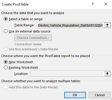
- Click the “Insert” tab and choose “PivotTable”.
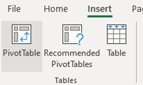
- Select “New Worksheet”, then click “OK”.
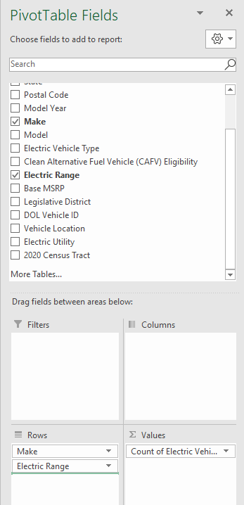
- Drag and drop the fields you want to see as rows, columns, and values in your pivot table.
2. Filtering by Range:
- Now, to filter based on a specific range, ensure the field with the desired range is included in the “Rows” area.
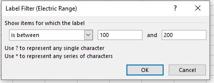
- Right-click on any value within that field and select “Label Filters”.
- Choose “Between” from the options and enter your desired range (e.g., “100” and “200”).
- Click “OK” to apply the filter.
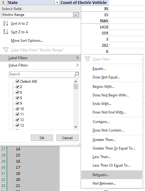
Voila! Your pivot table now displays only the values that fall within your chosen range.
Pro Tips:
- You can apply multiple filters simultaneously by repeating step 2 for different fields.
- Use the “Top 10” filter to easily identify the highest or lowest values.
- Don’t forget to experiment with different filtering options to explore your data from various angles.
By mastering pivot table filtering, you unlock a powerful tool for transforming vast amounts of data into actionable insights. So go forth and explore!